
Working with digital sound begins with an understanding of sound as a physical phenomenon. The sounds we hear are the result of vibrations of objects – for example, the human vocal chords, or the metal strings and wooden body of a guitar. In general, without the influence of a specific sound vibration, air molecules move around randomly. A vibrating object pushes against the randomly-moving air molecules in the vicinity of the vibrating object, causing them first to crowd together and then to move apart. The alternate crowding together and moving apart of these molecules in turn affects the surrounding air pressure. The air pressure around the vibrating object rises and falls in a regular pattern, and this fluctuation of air pressure, propagated outward, is what we hear as sound.
Sound is often referred to as a wave, but we need to be careful with the commonly-used term “sound wave,” as it can lead to a misconception about the nature of sound as a physical phenomenon. On the one hand, there’s the physical wave of energy passed through a medium as sound travels from its source to a listener. (We’ll assume for simplicity that the sound is traveling through air, although it can travel through other media.) Related to this is the graphical view of sound, a plot of air pressure amplitude at a particular position in space as it changes over time. For single-frequency sounds, this graph takes the shape of a “wave,” as shown in Figure 2.1. More precisely, a single-frequency sound can be expressed as a sine function and graphed as a sine wave (as we’ll describe in more detail later). Let’s see how these two things are related.
[wpfilebase tag=file tpl=supplement /]
First, consider a very simple vibrating object – a tuning fork. When the tuning fork is struck, it begins to move back and forth. As the prong of the tuning fork vibrates outward (in Figure 2.2), it pushes the air molecules right next to it, which results in a rise in air pressure corresponding to a local increase in air density. This is called compression. Now, consider what happens when the prong vibrates inward. The air molecules have more room to spread out again, so the air pressure beside the tuning fork falls. The spreading out of the molecules is called decompression or rarefaction. A wave of rising and falling air pressure is transmitted to the listener’s ear. This is the physical phenomenon of sound, the actual sound wave.
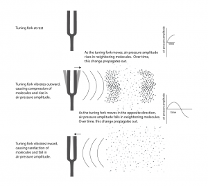
Assume that a tuning fork creates a single-frequency wave. Such a sound wave can be graphed as a sine wave, as illustrated in Figure 2.1. An incorrect understanding of this graph would be to picture air molecules going up and down as they travel across space from the place in which the sound originates to the place in which it is heard. This would be as if a particular molecule starts out where the sound originates and ends up in the listener’s ear. This is not what is being pictured in a graph of a sound wave. It is the energy, not the air molecules themselves, that is being transmitted from the source of a sound to the listener’s ear. If the wave in Figure 2.1 is intended to depict a single-frequency sound wave, then the graph has time on the x-axis (the horizontal axis) and air pressure amplitude on the y-axis. As described above, the air pressure rises and falls. For a single-frequency sound wave, the rate at which it does this is regular and continuous, taking the shape of a sine wave.
Thus, the graph of a sound wave is a simple sine wave only if the sound has only one frequency component in it – that is, just one pitch. Most sounds are composed of multiple frequency components – multiple pitches. A sound with multiple frequency components also can be represented as a graph which plots amplitude over time; it’s just a graph with a more complicated shape. For simplicity, we sometimes use the term “sound wave” rather than “graph of a sound wave” for such graphs, assuming that you understand the difference between the physical phenomenon and the graph representing it.
The regular pattern of compression and rarefaction described above is an example of harmonic motion, also called harmonic oscillation. Another example of harmonic motion is a spring dangling vertically. If you pull on the bottom of the spring, it will bounce up and down in a regular pattern. Its position – that is, its displacement from its natural resting position – can be graphed over time in the same way that a sound wave’s air pressure amplitude can be graphed over time. The spring’s position increases as the spring stretches downward, and it goes to negative values as it bounces upwards. The speed of the spring’s motion slows down as it reaches its maximum extension, and then it speeds up again as it bounces upwards. This slowing down and speeding up as the spring bounces up and down can be modeled by the curve of a sine wave. In the ideal model, with no friction, the bouncing would go on forever. In reality, however, friction causes a damping effect such that the spring eventually comes to rest. We’ll discuss damping more in a later chapter.
Now consider how sound travels from one location to another. The first molecules bump into the molecules beside them, and they bump into the next ones, and so forth as time goes on. It’s something like a chain reaction of cars bumping into one another in a pile-up wreck. They don’t all hit each other simultaneously. The first hits the second, the second hits the third, and so on. In the case of sound waves, this passing along of the change in air pressure is called sound wave propagation. The movement of the air molecules is different from the chain reaction pile up of cars, however, in that the molecules vibrate back and forth. When the molecules vibrate in the direction opposite of their original direction, the drop in air pressure amplitude is propagated through space in the same way that the increase was propagated.
Be careful not to confuse the speed at which a sound wave propagates and the rate at which the air pressure amplitude changes from highest to lowest. The speed at which the sound is transmitted from the source of the sound to the listener of the sound is the speed of sound. The rate at which the air pressure changes at a given point in space – i.e., vibrates back and forth – is the frequency of the sound wave. You may understand this better through the following analogy. Imagine that you’re watching someone turn a flashlight on and off, repeatedly, at a certain fixed rate in order to communicate a sequence of numbers to you in binary code. The image of this person is transmitted to your eyes at the speed of light, analogous to the speed of sound. The rate at which the person is turning the flashlight on and off is the frequency of the communication, analogous to the frequency of a sound wave.
The above description of a sound wave implies that there must be a medium through which the changing pressure propagates. We’ve described sound traveling through air, but sound also can travel through liquids and solids. The speed at which the change in pressure propagates is the speed of sound. The speed of sound is different depending upon the medium in which sound is transmitted. It also varies by temperature and density. The speed of sound in air is approximately 1130 ft/s (or 344 m/s). Table 2.1 shows the approximate speed in other media.
[table caption=”Table 2.1 The Speed of sound in various media” colalign=”center|center|center” width=”80%”]
Medium,Speed of sound in m/s, Speed of sound in ft/s
“air (20° C, which is 68° F)”,344,”1,130″
“water (just above 0° C, which is 32° F)”,”1,410″,”4,626″
glass,”approximately 4,000~~(depending on type of glass)”,”approximately 13,200″
[aside width=”75px”]
feet = ft
seconds = s
meters = m
[/aside]
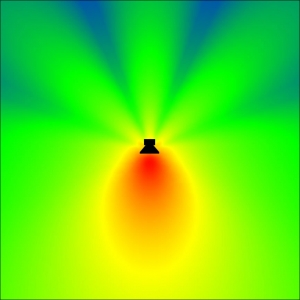
For clarity, we’ve thus far simplified the picture of how sound propagates. Figure 2.2 makes it look as though there’s a single line of sound going straight out from the tuning fork and arriving at the listener’s ear. In fact, sound radiates out from a source at all angles in a sphere. Figure 2.3 shows a top-view image of a real sound radiation pattern, generated by software that uses sound dispersion data, measured from an actual loudspeaker, to predict how sound will propagate in a given three-dimensional space. In this case, we’re looking at the horizontal dispersion of the loudspeaker. Colors are used to indicate the amplitude of sound, going highest to lowest from red to yellow to green to blue. The figure shows that the amplitude of the sound is highest in front of the loudspeaker and lowest behind it. The simplification in Figure 2.2 suffices to give you a basic concept of sound as it emanates from a source and arrives at your ear. Later, when we begin to talk about acoustics, we’ll consider a more complete picture of sound waves.
Sound waves are passed through the ear canal to the eardrum, causing vibrations which pass to little hairs in the inner ear. These hairs are connected to the auditory nerve, which sends the signal onto the brain. The rate of a sound vibration – its frequency – is perceived as its pitch by the brain. The graph of a sound wave represents the changes in air pressure over time resulting from a vibrating source. To understand this better, let’s look more closely at the concept of frequency and other properties of sine waves.
We assume that you have some familiarity with sine waves from trigonometry, but even if you don’t, you should be able to understand some basic concepts of this explanation.
A sine wave is a graph of a sine function . In the graph, the x-axis is the horizontal axis, and the y-axis is the vertical axis. A graph or phenomenon that takes the shape of a sine wave – oscillating up and down in a regular, continuous manner – is called a sinusoid.
In order to have the proper terminology to discuss sound waves and the corresponding sine functions, we need to take a little side trip into mathematics. We’ll first give the sine function as it applies to sound, and then we’ll explain the related terminology.
[equation caption=”Equation 2.1″]A single-frequency sound wave with frequency f , maximum amplitude A, and phase θ is represented by the sine function
$$!y=A\sin \left ( 2\pi fx+\theta \right )$$
where x is time and y is the amplitude of the sound wave at time x.[/equation]
[wpfilebase tag=file tpl=supplement /]
Single-frequency sound waves are sinusoidal waves. Although pure single-frequency sound waves do not occur naturally, they can be created artificially by means of a computer. Naturally occurring sound waves are combinations of frequency components, as we’ll discuss later in this chapter.
The graph of a sound wave is repeated Figure 2.4 with some of its parts labeled. The amplitude of a wave is its y value at some moment in time given by x. If we’re talking about a pure sine wave, then the wave’s amplitude, A, is the highest y value of the wave. We call this highest value the crest of the wave. The lowest value of the wave is called the trough. When we speak of the amplitude of the sine wave related to sound, we’re referring essentially to the change in air pressure caused by the vibrations that created the sound. This air pressure, which changes over time, can be measured in Newtons/meter 2 or, more customarily, in decibels (abbreviated dB), a logarithmic unit explained in detail in Chapter 4. Amplitude is related to perceived loudness. The higher the amplitude of a sound wave, the louder it seems to the human ear.
In order to define frequency, we must first define a cycle. A cycle of a sine wave is a section of the wave from some starting position to the first moment at which it returns to that same position after having gone through its maximum and minimum amplitudes. Usually, we choose the starting position to be at some position where the wave crosses the x-axis, or zero crossing, so the cycle would be from that position to the next zero crossing where the wave starts to repeat, as shown in Figure 2.4.
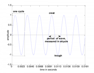
The frequency of a wave, f, is the number of cycles per unit time, customarily the number of cycles per second. A unit that is used in speaking of sound frequency is Hertz, defined as 1 cycle/second, and abbreviated Hz. In Figure 2.4, the time units on the x-axis are seconds. Thus, the frequency of the wave is 6 cycles/0.0181 seconds » 331 Hz. Henceforth, we’ll use the abbreviation s for seconds and ms for milliseconds.
Frequency is related to pitch in human perception. A single-frequency sound is perceived as a single pitch. For example, a sound wave of 440 Hz sounds like the note A on a piano (just above middle C). Humans hear in a frequency range of approximately 20 Hz to 20,000 Hz. The frequency ranges of most musical instruments fall between about 50 Hz and 5000 Hz. The range of frequencies that an individual can hear varies with age and other individual factors.
The period of a wave, T, is the time it takes for the wave to complete one cycle, measured in s/cycle. Frequency and period have an inverse relationship, given below.
[equation caption=”Equation 2.2″]Let the frequency of a sine wave be and f the period of a sine wave be T. Then
The period of the wave in Figure 2.4 is about three milliseconds per cycle. A 440 Hz wave (which has a frequency of 440 cycles/s) has a period of 1 s/440 cycles, which is about 0.00227 s/cycle. There are contexts in which it is more convenient to speak of period only in units of time, and in these contexts the “per cycle” can be omitted as long as units are handled consistently for a particular computation. With this in mind, a 440 Hz wave would simply be said to have a period of 2.27 milliseconds.
[wpfilebase tag=file tpl=supplement /]
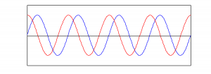
The phase of a wave, θ, is its offset from some specified starting position at x = 0. The sine of 0 is 0, so the blue graph in Figure 2.5 represents a sine function with no phase offset. However, consider a second sine wave with exactly the same frequency and amplitude, but displaced in the positive or negative direction on the x-axis relative to the first, as shown in Figure 2.5. The extent to which two waves have a phase offset relative to each other can be measured in degrees. If one sine wave is offset a full cycle from another, it has a 360 degree offset (denoted 360 o ); if it is offset a half cycle, is has a 180 o offset; if it is offset a quarter cycle, it has a 90 o offset, and so forth. In Figure 2.5, the red wave has a 90 o offset from the blue. Equivalently, you could say it has a 270 o offset, depending on whether you assume it is offset in the positive or negative x direction.
Wavelength, λ, is the distance that a single-frequency wave propagates in space as it completes one cycle. Another way to say this is that wavelength is the distance between a place where the air pressure is at its maximum and a neighboring place where it is at its maximum. Distance is not represented on the graph of a sound wave, so we cannot directly observe the wavelength on such a graph. Instead, we have to consider the relationship between the speed of sound and a particular sound wave’s period. Assume that the speed of sound is 1130 ft/s. If a 440 Hz wave takes 2.27 milliseconds to complete a cycle, then the position of maximum air pressure travels 1 cycle * 0.00227 s/cycle * 1130 ft/s in one wavelength, which is 2.57 ft. This relationship is given more generally in the equation below.
[equation caption=”Equation 2.3″]Let the frequency of a sine wave representing a sound be f, the period be T, the wavelength be λ, and the speed of sound be c. Then